
In this one, we shall obsess over plotting and LaTex. Microsoft Word enthusiasts, you have been warned!
So lets talk about scientific writing. It tends to be fussy. Very fussy. The font needs to be just right, the layout just perfect. Most journals will supply a “Guide for Authors” that rivals the size of typical journal papers. Have a look at this one for Applied Energy, or this one for Journal of Fluid Mechanics. Some others journals have simply given up, and in those journals, you will see figures with tiny font, and the font in the document will be different from that in the figure, they will have bit-mapped figures that are blurred out, etc.

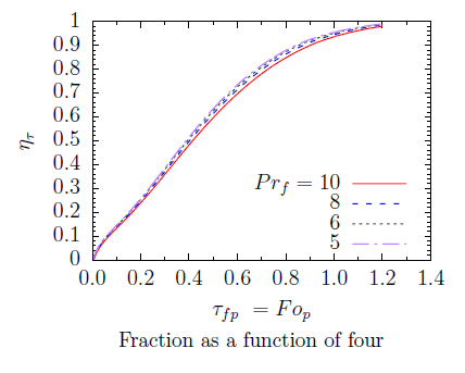
Why point fingers? Here’s Fig. 1 from one of my own papers that has this issue, some text from the paper is pasted below the figure, and you notice
that none of the font types/sizes match, and the overall effect is messy
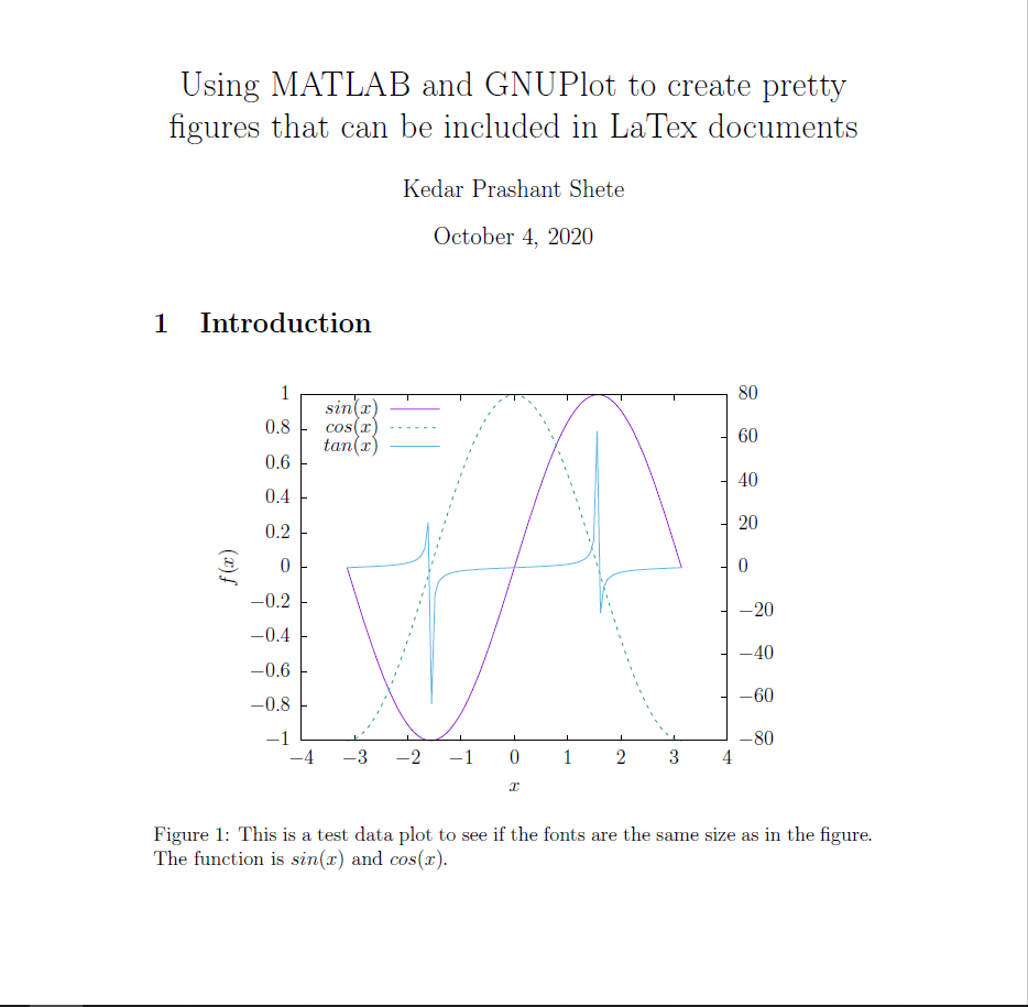
(I blurred out some text from the plots to protect the anonymity of my coauthors). Now compare that to Fig. 2, which does not have any of these problems.
The question is, how to go from making figures like Fig. 1 to figures like Fig. 2 ?
So what really separates a publication quality figure from the rest ? Omitting obvious stuff like axes labels, tick marks, legends, etc., here are some other points:
| Fig. 1 | Fig. 2 | |
|---|---|---|
| Vectorized format, the plot and text resize automatically with plot size | ❌ | ✅ |
| Plot font matches text | ❌ | ✅ |
| Plot font changes automatically to match text font | ❌ | ✅ |
| Pretty LaTex like font for figures | ❌ | ✅ |
Any plotting package worth its name will be able to deliver the first characteristic, which is a vectorized plot. These come in a variety of file formats, the most common being ‘.eps’ and ‘.tiff’. MATLAB will also provide “LaTex” font, although you have to trial-and-error the font size to match the text. But even a vectorized image from MATLAB won’t change font automatically with text. That’s because the font information is not provided separately in the eps figure from MATLAB, instead the letters are just a geometry like other stuff in the plot. Apparently, this is to protect proprietary font information(which does not make sense for LaTex, as the font is open source). So how do we get all characteristics ?
Thats where LaTex and GNUPlot come in. GNUPlot, Inkscape and some other softwares provide the option to export a figure and its text separately, as a figure.eps and figure.tex file. You include the figure.tex file when you compile your paper.tex, and it takes the figure.eps figure, puts the text content contained in figure.tex on top of it and generates a figure with all four characteristics in the table. If you resize the figure.tex in paper.tex, or change font of paper.tex, or size, and hey presto!, everything in the figure adjusts to match the main text automatically! Sounds too good to be true, right? It did to me first, I was used to making and remaking figures in Excel/MATLAB.
Well, this is done using what’s called “epslatex” plotting terminal of GNUPlot. GNUPlot is a plotting package with a certain pedigree, and has been used by researchers over the years as it seems to do everything. It is a command line tool(there might be a GUI, but I don’t recommend), and works by reading data from space/comma separated column text files. The whole work flow is based on reading data from simple text files and plotting it. So what outputs these text files ? GNUPlot can do certain calculations, and in that sense is a programming language. But the syntax can be daunting if you want to do anything more than addition and subtraction. It is really best if you do all the calculations in another language, output the text file and then use GNUPlot just for what it does best, which is plotting.
As an example, I show a MATLAB script to plot a a few trigonometric functions. The initial bit is generating the data, this step can be any postprocessing you are doing with simulation data, anything at all. Then I write it to a file. The rest of the script writes a GNUPlot script and then runs it. The “epslatex” option in “set terminal” gets us this “eps + tex” format that has all the characteristics we would want from a good figure. Adding a “standalone” flag will make the “tex” file self compilable, as in it is self sufficient and can be compiled with pdflatex. Here, I have omitted that flag as I am including the “tex” file in “document.tex”. I attached all files for clarity, happy plotting!